Reconstructing 1938 San Francisco from Aerial Images

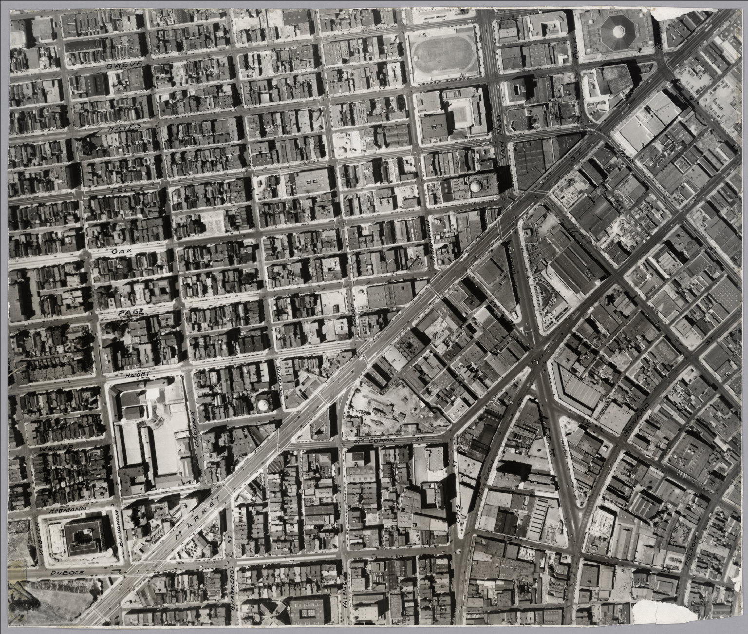
This winter I took Silvio Savarese’s course on 3D computer vision through the Stanford Center for Professional Development. For my final project, I worked with Justin Manley to reconstruct a 3D topography of 1938 San Francisco from a series of aerial photographs taken by Harrison Ryker, available digitally through the Rumsey Map Collection at Stanford. I highly recommend checking out the full collection of images. It’s like perusing a 1938 satellite view of the city.

We focused our efforts on regions of the city that are covered by at least two distinct images, so that we could use stereo vision techniques to recover depth information. The photographs are in remarkably good shape for having been taken the better part of a century ago but are still difficult to work with because of their age and history. They are available as GeoTIFF files, which include geographic metadata that approximately maps the image pixels to the Earth’s latitude and longitude. (I use approximately here because this mapping ignores the variation in altitude and 3D structure within a photograph, and because the georectification process seems to have been done by hand and is frequently off by 10s of pixels.) Despite the inaccuracies, Justin wrote an effective C++ module that uses GDAL and CGAL to analyze the overlapped regions of a set of images and return masking patterns indicating the overlaps. This allows us to focus our analyses on the areas of interest.

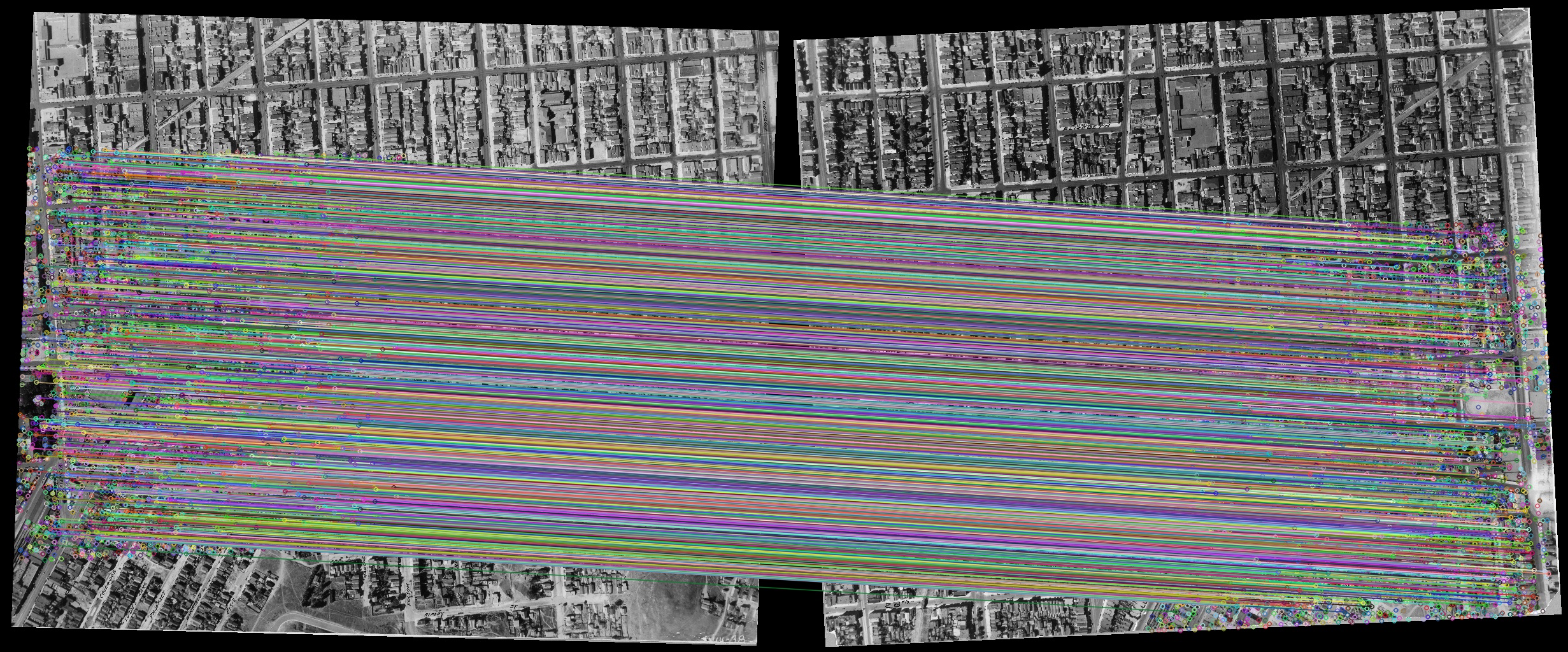
I’ve worked with the OpenCV library in the past, but this was my first chance to really dive in and see what a structure from motion pipeline looks like using the library. We started out using ORB keypoints to try and extract sparse point correspondences between the images but found that ORB’s affinity for edges meant that keypoints were strongly drawn to the artefacts in the images, such as tears, rips, and what seem to be street names that Mr. Ryker labeled by hand in dark ink. These don’t give us any useful information about the structure of the scene, so we experimented with other keypoint strategies until we hit on the more recently-developed AKAZE features. AKAZE is the accelerated version of the KAZE algorithm described here. For the Ryker dataset, it delivers a set of points that is much more evenly distributed in space when compared with ORB, perhaps because of the algorithm’s much-touted “nonlinear scale” representation; whereas with ORB, many keypoints of different scales can all be collocated on the same edge, AKAZE seems to consider each edge once.

Equipped with keypoint matches between images, we used the geotiff metadata to establish an approximate guess for the location of the points in 3D space. This guess assumes the structure in the images is completely flat, and that the cameras are oriented 2000m in the air facing directly downward. We then used the sba library to perform a bundle adjustment on the points. This adjustment refines the initial point location estimates using the Levenburg-Marquardt algorithm. The algorithm minimizes the reprojection errors of the 3D point estimates into the 2D images through dynamic camera models. There are many bundle adjustment libraries available, but SBA seems to be the best-suited for cases where the 3D point locations, 6D camera poses, and 5D camera intrinsic matrices are all unknown to begin with (many of the bundle adjustment libraries we looked at assume that the camera intrinsics are known, either through the manufacturer or a calibration process). Aside from the initial state estimate of all the system parameters and the locations of all the observed points in their respective images, the SBA library requires a reprojection function that calculates the reprojection of the 3D points into the image planes (for comparison with the observations) and a Jacobian function that calculates how the reprojections should change if the model parameters are varied. For these functions, we had good luck with the sample code provided with the SBA library, which needed only minor modifications to run with our dataset. Below to the left you can see the areas of SF’s Twin Peaks neighborhood that are covered by at least two images in the set, and to the right the corresponding point data that we extracted. Our initial point estimates are in red, overlaid with the bundle-adjusted points in blue.

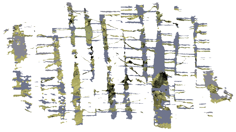
Justin put together a great analysis of our resulting point cloud and how it compares with a modern elevation map of San Francsicso, which you can read over on the project github page You can also read our project report here, although it doesn’t include the latest analyses. Ultimately, our reconstruction seems closer to the ground truth elevation than does a flat plane, but there’s still a good amount of work to do to get the point cloud within a reasonable (say, sub-10 meter) error. In particular, it seems the point reconstruction doesn’t have nearly the variation in elevation that it should; it is much flatter in general than the geographic elevation profile. I have some thoughts on ways to improve the project, which we will try and implement when we next have time. In the meantime it’s interesting to look at the full reconstruction, shown below in silver with a modern elevation profile of SF in gold.